The Fidelity–Limit Theorem
A closed-form predictability horizon for chaotic systems, introduced by Debosmita Sarkar. It answers a precise question: how long can a simulation of a chaotic system — like the solar system — stay within a chosen tolerance of reality before error growth makes it unreliable?
In brief
The Fidelity–Limit Theorem is a closed-form result that gives the exact time a simulation of a chaotic system stays within a chosen tolerance of reality. A predictability horizon is the length of time a chaotic simulation remains trustworthy before error growth makes it unreliable, and the measurement ceiling is the limit beyond which prediction depends on how well reality was measured, not on computing power. The theorem states that the simulated positional error stays below a tolerance $\Delta_{\mathrm{tol}}$ for all $t \le t_{\mathrm{lim}}$, where
$$t_{\mathrm{lim}} = \frac{1}{\lambda}\,\ln\!\left[\frac{\Delta_{\mathrm{tol}}}{\Delta_0 + C h^{p}/\lambda}\right].$$
It binds five quantities: the integrator order $p$, step size $h$, the largest Lyapunov exponent $\lambda$, the initial measurement uncertainty $\Delta_0$, and the tolerance $\Delta_{\mathrm{tol}}$. Its central consequence — the measurement ceiling — is that beyond a computable point, prediction is limited by how well reality is measured, not by how much computing power you have.
The error-growth law
Two mechanisms act on the error $\Delta(t)$ simultaneously: the chaotic flow amplifies existing error at rate $\lambda$, and each integrator step injects local truncation error at rate $C h^{p}$ per unit time. This gives a linear ODE with an exact solution.
Lemma (Error growth)
$\Delta(t)$ obeys $\dot\Delta = \lambda\Delta + C h^{p}$ with $\Delta(0)=\Delta_0$, whose exact solution is
$$\Delta(t) = \left(\Delta_0 + \frac{C h^{p}}{\lambda}\right) e^{\lambda t} - \frac{C h^{p}}{\lambda}.$$
Theorem (Predictability horizon)
Setting $\Delta(t_{\mathrm{lim}}) = \Delta_{\mathrm{tol}}$ and solving gives the closed-form horizon above.
Two regimes
Corollary — logarithmic return on computation
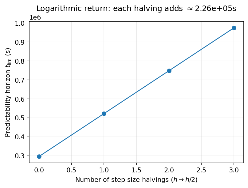
In the integrator-dominated regime, halving the step size $h$ extends the horizon by only $p\ln 2/\lambda$. Exponential computational effort buys merely linear predictive time — computation cannot outrun chaos.
Corollary — the measurement ceiling
When the initial uncertainty dominates ($\Delta_0 \gg Ch^p/\lambda$),
$$t_{\mathrm{lim}} \;\longrightarrow\; \frac{1}{\lambda}\ln\!\frac{\Delta_{\mathrm{tol}}}{\Delta_0},$$
independent of the integrator. No amount of computation extends prediction beyond this ceiling; only a better measurement of reality can. This is the most defensible and far-reaching consequence of the theorem.
Worked example: the ~100-million-year horizon
The theorem earns trust by reproducing a known result it was not fitted to. Inserting the canonical inner-solar-system values — Lyapunov time $1/\lambda \approx 5$ Myr, initial uncertainty $\Delta_0 \approx 15$ m, and tolerance $\Delta_{\mathrm{tol}} \approx 1$ AU $\approx 1.496\times10^{11}$ m — gives $\Delta_{\mathrm{tol}}/\Delta_0 \approx 10^{10}$, $\ln(10^{10}) \approx 23$, and
$$t_{\mathrm{lim}} \approx 5~\text{Myr}\times 23 \approx 115~\text{Myr},$$
landing squarely on the established ~100 Myr predictability horizon of the solar system. It is a consistency check the theorem passes, not a fit.
Numerical confirmation
Using a Lyapunov exponent measured independently ($\lambda = 6.126\times10^{-6}\,\mathrm{s}^{-1}$), each halving of the step size adds a constant 226 293 s to the horizon — matching the predicted $p\ln2/\lambda$ to four significant figures with no free parameters. This tests the theorem as a falsifiable prediction and confirms it.
Frequently asked questions
What is the Fidelity–Limit Theorem?
The Fidelity–Limit Theorem, introduced by Debosmita Sarkar, gives an explicit closed-form predictability horizon $t_{\mathrm{lim}} = \frac{1}{\lambda}\ln[\Delta_{\mathrm{tol}}/(\Delta_0 + C h^p/\lambda)]$, binding the integrator order, step size, Lyapunov exponent, measurement uncertainty, and tolerance.
What is the measurement ceiling?
Once numerical errors fall below the initial measurement uncertainty, the horizon becomes $\frac{1}{\lambda}\ln(\Delta_{\mathrm{tol}}/\Delta_0)$, independent of the integrator. No amount of computation extends prediction past this ceiling — only a better measurement of reality can.
How far into the future can the solar system be predicted?
About 100 million years. With a Lyapunov time near 5 million years, initial uncertainty ~15 m, and a 1 AU tolerance, the theorem gives ≈115 million years, matching the established limit.
Read the full derivation and proofs in the complete paper, or see how the theorem is tested in the gravitational world simulator.