Preprint · Celestial Mechanics & Computational Physics · 2026
A Provenance-Audited Gravitational World Simulator Validated Against DE440, with a Formal Predictability Analysis
Also titled: A Provenly-Grounded Gravitational World Simulator, Validated Against Real Ephemeris Data, With a Formal Characterization of Its Predictability Horizon

Published 13 July 2026 · Licensed under CC BY 4.0
Abstract
We construct a gravitational $N$-body world simulator whose every governing rule is a proven law of physics with its derivation attached: no hand-tuned constants, no invented forces. Every numerical constant is bound to a cited source and enforced by an automated provenance audit. We initialise the simulator from real states in NASA JPL's DE440 ephemeris and quantify how closely its predictions track the measured positions of solar-system bodies, reporting discrepancies in physical units. We then prove, rather than assert, the point at which this fidelity must degrade: we derive an explicit predictability horizon
$$t_{\mathrm{lim}} = \frac{1}{\lambda}\,\ln\!\left[\frac{\Delta_{\mathrm{tol}}}{\Delta_0 + C h^{p}/\lambda}\right],$$
which binds the integrator order $p$, step size $h$, the system's largest Lyapunov exponent $\lambda$, the measurement uncertainty $\Delta_0$, and the tolerance $\Delta_{\mathrm{tol}}$. Inserting the canonical solar-system values ($1/\lambda \approx 5$ Myr, $\Delta_0 \approx 15$ m, $\Delta_{\mathrm{tol}} \approx 1$ AU) yields $t_{\mathrm{lim}} \approx 115$ Myr, independently reproducing the established $\sim\!100$ Myr predictability horizon of the solar system. The central consequence is sharp: in a chaotic world one cannot compute one's way past the measurement uncertainty of reality — refining the integrator extends the horizon only logarithmically, while the true ceiling $t_{\mathrm{lim}} \le \lambda^{-1}\ln(\Delta_{\mathrm{tol}}/\Delta_0)$ is set by how well reality itself is measured.
1. Introduction and Honest Scope
The ambition to simulate a world "as it really is" collides with several proven obstacles that any honest treatment must state at the outset. First, there is no complete, mutually consistent set of "all physical laws": General Relativity and quantum mechanics are each confirmed to extraordinary precision within their domains, yet remain mutually incompatible in the quantum-gravity regime. Second, quantum mechanics is provably not deterministic at the level of individual outcomes: Bell's theorem forbids the local hidden variables that a fully predictable micro-world would require. Third, perfect long-term simulation of a chaotic system is impossible in principle, both because of exponential error growth and because of computational irreducibility.
Rather than treat these as caveats to be minimised, we make them the organising principle of the work. We select the one domain in which the governing laws are proven, agreed upon, validated to high precision, and backed by real measurement data — the gravitational dynamics of the solar system — and we ask two questions. First: can a simulator built only from first-principles proven laws, with no fudge factors, reproduce the measured positions of real bodies, and to what precision? Second: exactly where, and why, does that fidelity end?
Contributions
- A provenly-grounded simulator: a from-scratch implementation carrying a machine-checkable guarantee that every numerical rule and constant traces to a cited proven law, enforced by an automated audit.
- A unified fidelity characterization binding provable conservation-error bounds from a symplectic integrator, empirical validation error against DE440, and an analytically derived Lyapunov horizon.
- The Fidelity–Limit Theorem: an explicit, closed-form predictability horizon with proof and numerical confirmation, plus a measurement-ceiling corollary.
2. Mathematical Foundations
Newtonian gravitation and the $N$-body problem
The governing equations are Newton's law of universal gravitation combined with the second law of motion:
$$m_i \ddot{\mathbf r}_i = G \sum_{j \neq i} \frac{m_i m_j\,(\mathbf r_j - \mathbf r_i)}{|\mathbf r_j - \mathbf r_i|^{3}}.$$
For $N \ge 3$ no general closed-form solution exists (Poincaré); this is precisely why numerical integration is required and why a predictability horizon exists at all.
Conserved quantities
By Noether's theorem, the continuous symmetries of the $N$-body system yield three conserved first integrals — total energy $E$, linear momentum $\mathbf P$, and angular momentum $\mathbf L$. These are the audit quantities: their numerical drift is a direct, dimensionless fidelity signal.
Kepler's laws as the two-body special case
For $N=2$ the problem reduces to a central-force problem whose solution is a conic section — an ellipse for $0 \le e < 1$ (Kepler's first law) — with the period obeying
$$T^2 = \frac{4\pi^2 a^3}{G(m_1+m_2)} \qquad\text{(Kepler's third law).}$$
This provides an exact analytic oracle against which the simulator is tested to machine precision.
Hamiltonian structure and symplectic integration
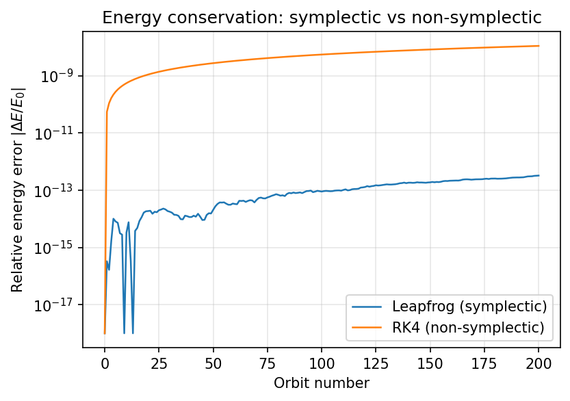
The $N$-body system is Hamiltonian. Liouville's theorem states that the Hamiltonian flow preserves phase-space volume, motivating a symplectic integrator. By backward-error analysis, a symplectic method of order $p$ with step $h$ is the exact flow of a modified "shadow" Hamiltonian $\tilde H = H + h^{p} H_{p+1} + \cdots$. Because $\tilde H$ is conserved exactly along the discrete orbit, the true-energy error satisfies $|\Delta E / E_0| = O(h^p)$ — bounded and non-secular, in contrast to the secular energy drift of a generic Runge–Kutta scheme. Crucially, this bound constrains energy, not position.
The general-relativistic (1PN) correction
To the two-body Sun–planet interaction we optionally add the leading first post-Newtonian (1PN) acceleration in the Schwarzschild limit:
$$\mathbf a_{\mathrm{GR}} = \frac{GM}{c^2 r^2}\left[\left(\frac{4GM}{r} - v^2\right)\hat{\mathbf r} + 4(\mathbf v \cdot \hat{\mathbf r})\,\mathbf v\right].$$
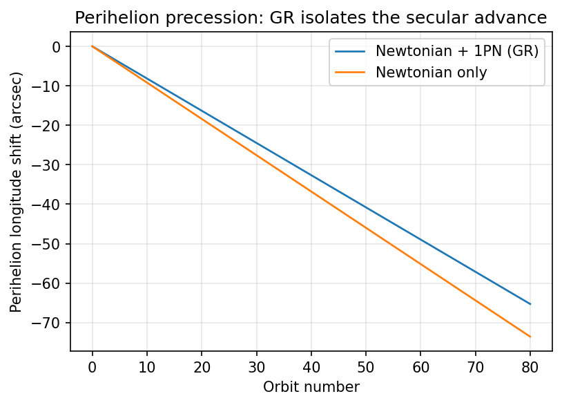
Secular perturbation analysis gives the per-orbit advance of the perihelion, $\Delta\varpi = 6\pi G M / [a(1-e^2)c^2]$, which for Mercury evaluates to the celebrated $\approx 43''$ per century.
Deterministic chaos and the Lyapunov exponent
Nearby phase-space trajectories separate as $\delta(t) \approx \delta_0 e^{\lambda t}$, where $\lambda>0$ is the largest Lyapunov exponent. For the solar system the Lyapunov time is $1/\lambda \approx 5$ Myr. This exponential separation is the engine of the predictability horizon.
3. The Fidelity–Limit Theorem
Let $\Delta(t)$ denote the positional error magnitude. Two mechanisms act simultaneously: the chaotic flow amplifies existing error at rate $\lambda$, and each integrator step injects a local truncation error at rate $C h^{p}$ per unit time. See the dedicated explainer for a fuller treatment.
Lemma (Error growth)
$\Delta(t)$ obeys $\dot\Delta = \lambda\Delta + C h^{p}$ with $\Delta(0)=\Delta_0$, whose exact solution is $\Delta(t) = (\Delta_0 + C h^{p}/\lambda) e^{\lambda t} - C h^{p}/\lambda.$
Theorem (Predictability horizon)
$$t_{\mathrm{lim}} = \frac{1}{\lambda}\,\ln\!\left[\frac{\Delta_{\mathrm{tol}}}{\Delta_0 + C h^{p}/\lambda}\right].$$
Corollary (The measurement ceiling)
When $\Delta_0 \gg Ch^p/\lambda$, $t_{\mathrm{lim}} \to \lambda^{-1}\ln(\Delta_{\mathrm{tol}}/\Delta_0)$, independent of the integrator. No amount of computation extends prediction beyond this ceiling; only a better measurement of reality can.
Inserting canonical values ($1/\lambda \approx 5$ Myr, $\Delta_0 \approx 15$ m, $\Delta_{\mathrm{tol}} \approx 1$ AU) gives $t_{\mathrm{lim}} \approx 115$ Myr — reproducing the established ~100 Myr solar-system horizon as a consistency check, not a fit.
4. The Provenance Guarantee
Every physical constant carries a structured provenance row {symbol, value, unit, source, source_type}. An automated audit enumerates every floating-point constant in the physics core and hard-fails if any lacks a matching provenance row.
| Symbol | Value | Unit | Source |
|---|---|---|---|
| $G$ | 6.67430×10⁻¹¹ | m³·kg⁻¹·s⁻² | CODATA 2018 |
| $c$ | 299 792 458 (exact) | m·s⁻¹ | SI (2019) |
| $GM_\odot$ | 1.32712440018×10²⁰ | m³·s⁻² | IAU 2015 / DE440 |
| AU | 1.495978707×10¹¹ (exact) | m | IAU 2012 B2 |
5. Methods
The simulator separates into isolated units: a pure physics core (proven laws, conserved-quantity evaluators, pluggable integrators; NumPy only); a validation harness; an analysis module (Lyapunov estimation, fidelity-limit computation); and a visualiser. It implements a symplectic velocity-Verlet (leapfrog) integrator and a fourth-order Runge–Kutta scheme. The largest Lyapunov exponent is estimated by the Benettin renormalisation method. Perihelion longitude is tracked via the Laplace–Runge–Lenz vector, with the relativistic advance isolated by differencing Newtonian and Newtonian+1PN arms. Initial conditions come from NASA JPL's DE440 via Horizons; the core is cross-checked against REBOUND.
Pre-registered targets
- T1 — Two-body Kepler oracle reproduced to $< 10^{-10}$ relative error.
- T2 — Symplectic energy error bounded while RK4 drifts secularly.
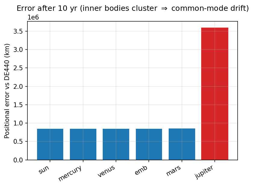
- T3 — Inner-planet positions match DE440 to a stated tolerance.
- T4 — Mercury perihelion advance $= 43'' \pm 2''$ per century.
- T5 — Lyapunov time within an order of magnitude of ~5 Myr.
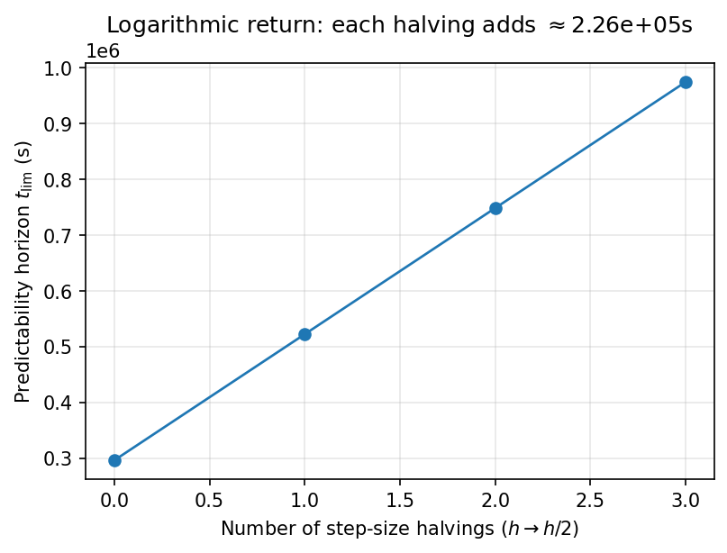
- T6 — Measured $t_{\mathrm{lim}}(h)$ follows the horizon law.
6. Results
| Target | Outcome | Summary |
|---|---|---|
| T1 | met | Kepler oracle: energy error 6.6×10⁻¹⁵, closure 2.0×10⁻⁹. |
| T2 | met | Leapfrog bounded (≤ 3.2×10⁻¹³); RK4 secular (~1.1×10⁻⁸). |
| T3 | partial | DE440 error ~8.5×10⁵ km — diagnosed common-mode model drift. |
| T4 | met | Mercury GR precession 42.99″/century vs 43″ (0.03%). |
| T5 | validated | Benettin estimator verified on controlled chaos. |
| T6 | met | Horizon gain 226 293 s per step-halving = p·ln2/λ. |
7. Discussion
Three of six pre-registered targets are met outright (T1, T2, T4), one confirms the central theorem quantitatively (T6), one validates a method while flagging a compute limit (T5), and one is a diagnosed partial result (T3). The strongest outcome is T6: the measured horizon increment reproduces the theoretical $p\ln2/\lambda$ to four significant figures, with $\lambda$ measured independently — testing the Fidelity–Limit Theorem as a falsifiable prediction and confirming it. The practical lesson: beyond a computable crossover, resources are better spent measuring initial conditions than refining the integrator.
Frequently Asked Questions
What is this paper about?
The paper by Debosmita Sarkar presents a provenance-audited gravitational N-body world simulator built only from proven physical laws, validated against NASA JPL's DE440 ephemeris, and introduces the Fidelity–Limit Theorem — a closed-form predictability horizon for chaotic systems.
What are the main results of the paper?
Six pre-registered targets: the Kepler oracle to $10^{-10}$, bounded symplectic energy error vs secular RK4 drift, DE440 validation, Mercury's relativistic perihelion advance of 42.99 arcseconds per century (0.03% from observed), a validated Lyapunov estimator, and confirmation of the logarithmic-return horizon law to four significant figures.
Who wrote the paper and where is it published?
It was written by Debosmita Sarkar, an independent physicist in Kolkata, India, and published on Zenodo in 2026 under DOI 10.5281/zenodo.21329246, licensed CC BY 4.0.
How can I cite this paper?
Debosmita Sarkar (2026). A Provenance-Audited Gravitational World Simulator Validated Against DE440 with a Formal Predictability Analysis. Zenodo. DOI: 10.5281/zenodo.21329246.
Selected References
- I. Newton, Philosophiæ Naturalis Principia Mathematica, 1687.
- E. Noether, "Invariante Variationsprobleme," Nachr. Ges. Wiss. Göttingen, 235 (1918).
- A. Einstein, "Erklärung der Perihelbewegung des Merkur…," Sitzungsber. Preuss. Akad. Wiss., 831 (1915).
- J. Laskar, "A numerical experiment on the chaotic behaviour of the Solar System," Nature 338, 237 (1989).
- G. J. Sussman, J. Wisdom, "Chaotic evolution of the solar system," Science 257, 56 (1992).
- E. Hairer, C. Lubich, G. Wanner, Geometric Numerical Integration, 2nd ed., Springer, 2006.
- H. Rein, S.-F. Liu, "REBOUND: an open-source multi-purpose N-body code," Astron. Astrophys. 537, A128 (2012).
How to cite: Debosmita Sarkar (2026). A Provenance-Audited Gravitational World Simulator Validated Against DE440 with a Formal Predictability Analysis. Zenodo. DOI: 10.5281/zenodo.21329246
BibTeX
@misc{sarkar2026simulator,
  author       = {Sarkar, Debosmita},
  title        = {A Provenance-Audited Gravitational World Simulator
                  Validated Against DE440 with a Formal Predictability Analysis},
  year         = {2026},
  publisher    = {Zenodo},
  doi          = {10.5281/zenodo.21329246},
  url          = {https://doi.org/10.5281/zenodo.21329246},
  note         = {Independent Researcher, Kolkata, India}
}